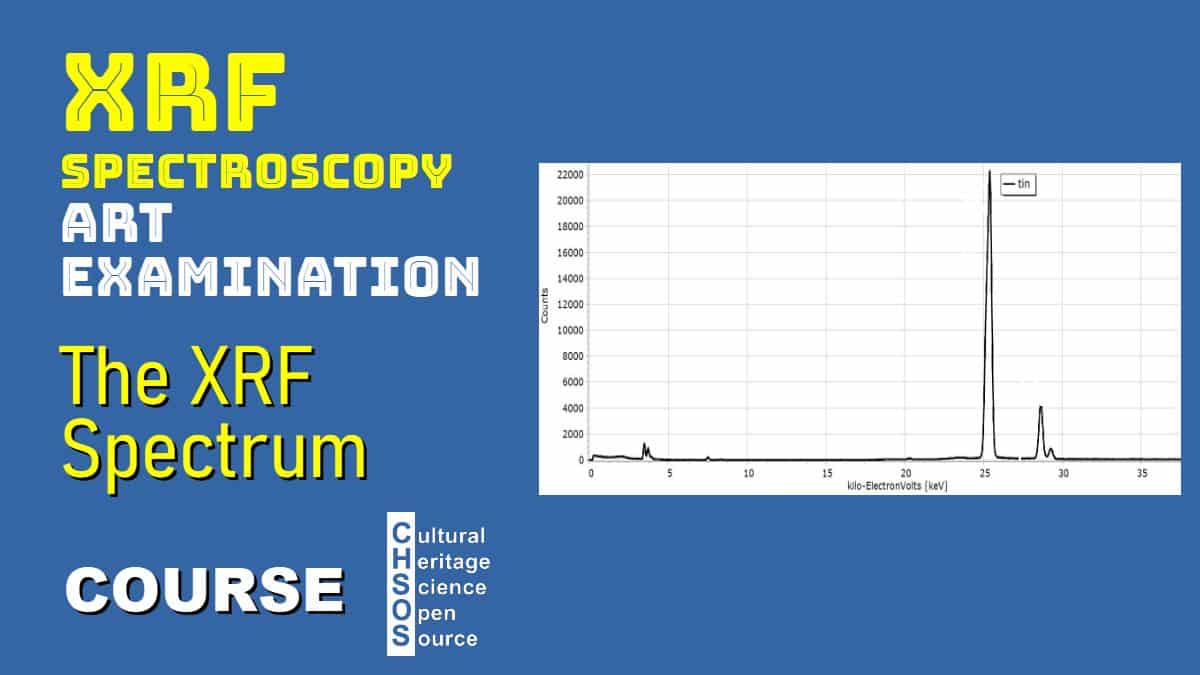
- Identify the multiple peaks (e.g., Kα, Kβ, Lα, Lβ) in an XRF spectrum and understand their origin.
- Understand the concepts of series probability and cascade effects in generating XRF peaks.
- Compare linear and logarithmic scales for visualizing XRF spectra.
- Example XRF spectrum of tin.
- Introduction to XRF Spectrum Features
- Explain why multiple peaks appear in an XRF spectrum for each element.
- Use the tin spectrum to introduce Kα, Kβ, Lα, and Lβ peaks.
- Series Probability and Cascade Effect
- Discuss how transitions between shells (e.g., K, L, M) result in multiple peaks.
- Explain the cascade effect and its role in producing additional X-ray lines.
- Visualization of XRF Spectra
- Compare linear and logarithmic scales for representing spectra.
- Highlight how logarithmic scales help reveal weaker lines, such as Lα and Lβ.


Free Course: XRF Spectroscopy for Art Examination
The course XRF Spectroscopy for Art Examination introduces conservators, art historians, and scientists with interest in Art to the principles and practical applications of X-ray fluorescence (XRF) spectroscopy in the examination of artworks. The course starts with basic principles of XRF and gradually explores its role in identifying materials and methods used in the creation and conservation of art.
Course Objectives
- Understand the fundamentals of XRF spectroscopy and how it applies to the analysis of art.
- Learn the key features and limitations of XRF for examining art and archaeology.
- Gain skills in interpreting XRF spectra to identify specific elements in paint layers, inks and metals.
Scientific Art Examination – Resources:
Getty Conservation Institute (GCI) – USA
The British Museum – Scientific Research Department – UK
Scientific Research Department – The Metropolitan Museum of Art, New York, USA
C2RMF (Centre de Recherche et de Restauration des Musées de France) – France
Rijksmuseum – Science Department – Netherlands


